|
|
|
|
Moscow Biosphere Model
A System of Models of the Global Biosphere Cycles of A.M. Tarko
Global Spatial Model of Carbon Dioxide Cycle in Terrestrial Ecosystems
1. Description of the Model
2. Pre-industrial State of Biosphere
3. Biosphere Dynamics under Impact of Industrial CO2 Emissions,
Deforestation and Soil Erosion
4. Zonal Distribution of CO2 absorption during industrial
period
5. Consequences of Global Warming for Russia
6. Carbon Dioxide Budget of Countries
Form to Download Data of CO2 Budget
of the Countries
7. Carbon Dioxide Budget of Biosphere
8. Estimation of performance Kyoto protocol to the UN
Framework Convention on climate change
9. Application the Control Theory in the Modeling
10. Final Remarks
| Investigation of the global carbon cycle in the biosphere is important.
On the one hand, carbon is a component of live and dead organic matter
of the biosphere and hence the indicator of ecological processes.
On the other hand, it is presented in the atmosphere as carbon dioxide
which defines the greenhouse effect and is a factor influencing the climate
of the planet. The next impotence is the nitrogen cycle.
A,M. Tarko developed system of models of global biogeochemical cycles in the biosphere including zero dimensional models of carbon and nitrogen cycle, and also spatial models of carbon cycle with a geographical grid 4x5 and 0.5x0.5o. The results of modeling biosphere dynamics in which the basic attention is given to the spatial cycle of carbon in the "Atmosphere - Terrestrial Plants - Soil" system are presented here. A simple carbon cycle model in the "Atmosphere - Ocean" system is added for full description the global cycle. The aim of modeling is to provide forecasts of atmospheric CO2 dynamics, to calculate CO2 parameters for the biosphere as a whole as well as for the individual countries and their ecosystems, and also to investigate the global role of terrestrial ecosystems in the compensation the anthropogenic impacts. In the model all land territory is divided
to into cells of the size 0.5x0.5o of a geographical grid. It
is supposed that in each cell there is a vegetation of one type according
to the chosen classification. Two kinds of classification of types are
used: 1. N.I. Bazilevich and L.E. Rodin and 2. J.S. Olson. The model is
described by system of ordinary nonlinear differential equations. The model
variables are quantities of carbon in the atmosphere, in live plants, and
in soil humus in each cell. A time unit accepted in the model is one year.
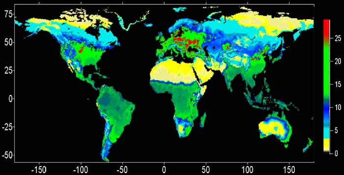
2. Pre-industrial State of the biosphere Computer map of annual production of the world vegetation at its pre-industrial state is shown below. The map is based on the annual production dependence of A.M. Tarko. |
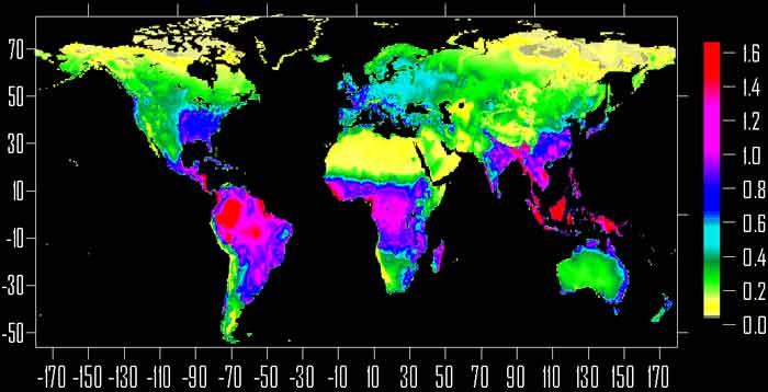
Computer map of annual production, kg C/(m2 yr)
| Computer map of humus at the pre-industrial state is shown below. Humus values calculations are based on the statistical estimation the dependence on temperature and precipitation. |
Computer map of soil humus, kg C/m2
|
Deforestation, and Soil Erosion We take into consideration the
following anthropogenic impacts on the biosphere resulting in CO2
growth in atmosphere: fossil fuel burning (industrial releases), cutting
down the forests, soil erosion resulting from wrong land use.
Calculation of dynamics of relative values of carbon in an the atmosphere,
Animated maps of plants biomass and humus changes in 1860-2050 are shown below.
Animated map of plants biomass changes in 1860-2050
Animated map of soil humus changes in 1860-2050
4. Zonal Distribution of CO2 Absorption during Industrial Period Consideration of the zonal distribution of CO2 exchange between the terrestrial ecosystems and the atmosphere during the industrial period shows that ecosystems of middle and high latitudes of the Northern hemisphere absorbed CO2 and ecosystems in the equatorial zone released CO2 . The greatest absorption occurred in middle latitudes of the Northern hemisphere where plentiful forest ecosystems are concentrated. Move from the middle latitudes to the equator, the closer the ecosystem or the country to are to the equator, the lesser is the degree of CO2 absorbing. And ecosystems of the equatorial zone were CO2 sinks. All ecosystems for this period absorbed more CO2 than they released.
Zonal distribution of CO2 absorption in 1860-1995 (Gt C/grad.). The whole territory of Russia during 1860-1995
was a CO2 sink though some ecosystems released CO2.
Forest ecosystems were most powerful CO2 absorbers. Grasslands
were CO2 sinks but at some territories were sources. Phytomass
was increased at all ecosystem types. Humus decreased at some grassland
ecosystems. Calculations show that now and in a future at the Russian territory
it will be increasing the annual plants production and phytomass. Russian
territory will absorb CO2 emissions. Quantity of humus will
be mainly increased. But at some territories which allocated at agricultural
zones mainly of southern regions humus will be decreased (see animated
map of humus changes).
A comparison of carbon budget of ecosystems in countries which are the greatest CO2 "producers" (annual production minus humus decomposition, minus deforestation, minus soil erosion) and the appropriate industrial releases in 1995 are shown in a figure. That year ecosystems of the whole the world and in each of the analyzed countries absorbed CO2 . The greatest industrial emissions were from territory of USA, China and Russia. The greatest CO2 absorption occurred in territories of Russia, Canada and the USA. In the majority of the countries industrial emissions exceeded ecosystem absorption. The exceptions were Canada, Australia, and Brazil where ecosystem CO2 absorption was more than industrial releases. It could be due to the rather large territory of the country and relatively small industrial releases.
Comparison of carbon absorption by ecosystems of the countries and industrial releases in 1995 (Gt C/ year)
Calculations show that the CO2 flows balance of in the world in 1995 was as follows. Deforestation - 1.08 Gt C/ year, Soil erosion - 0.91 Gt C/ year, Absorption by terrestrial ecosystems - 4.05 Gt C/ year, Absorption by ocean - 1.05 Gt C/ year, Remains in atmosphere - 3.30 Gt C/ year. 8. Estimation of performance of the Kyoto
protocol to the UN
In accordance to the Kyoto protocol (1997) to the UN Framework Convention on climate change all the countries should reduce the emissions of greenhouse gases by 2010 to a level of industrial CO2 emissions in 1990. We will consider the effects of various restrictions on reduction of CO2 emissions. The following scenarios were considered: 1. Above mentioned scenario of anthropogenic influences. 2. Scenario 1, but, after 2020, the industrial CO2 emissions become constant and equal to the value which was in 1990. 3. Scenario 1, but after 2010 industrial CO2 emissions become constant and equal to the value in 1990 (it corresponds to the Kyoto protocol). 4. Scenario 1, but after 2000 industrial CO2 emissions become constant and equal to the value in 1990 5. Scenario 1, but after 2000 industrial CO2 emissions stop. 6. Scenario 1, but after 1990 deforestation and erosion stop.
Results of calculation the Kyoto protocol scenario realization and other
scenarios of CO2 emissions reduction.
We see that emissions restrictions are effective.
According to scenario 1 CO2 concentration in atmosphere will
be raised by 1.82 times by 2050 in comparison with 1860. According to scenarios
2, 3, and 4 increases of CO2 concentration will be significantly
less: the CO2 growth will be 1.56, 1.47 and 1.42 times. It is
obviously that the delay of beginning to implement the Kyoto protocol for
10 years does not result in significant change in 2050.
Investigating the anthropogenic influences on the biosphere, it is important to establish not only what consequences of this or that economic strategy will be, but also what will be "a price" if we want to provide accepted values of biosphere parameters. Let us consider a task to set constant level of atmospheric CO2 after a given year. We are to determine what values of CO2 industrial emissions must be set to provide steady state of the atmospheric CO2. This was done using the control theory methods . Results of calculation show that in order to provide constant level of CO2 in the atmosphere it is necessary to significantly decrease amount of emissions.
Industrial releases at which the CO2 concentration in atmosphere remains constant after the given year (Gt C/ year) The models of global biosphere processes
can be compared with some kind of "universal recipient", since they combine
the approaches of many sciences: physics, chemistry, ecology, soil science,
geography, geochemistry, climatology, economy etc. However these models
are far from being "universal donor ". In other sciences, the amount of
consumers of global modeling results it is small. Results received by using
the global models enrich a science but practical application of global
models can be found among the decision-makers. Application of the results
of modeling is also possible in economic and social sciences. So, V.S.
Golubev (Institute of Lithosphere, Russian Academy of Sciences)
used the biosphere parameters calculated here to investigated indices
of social and natural development of various countries.
|
Copyright c A.M. Tarko, 1999, 2000, 2007
 .
.
 .
.