|
When an algorithm |
|
|
The concept of the complexity of an algorithm is measured as the time or storage space cost required to execute it in the worst or average case. This concept provides a mathematical definition for the rather vague term "hardness," which is sometimes used to characterize algorithms. |
|
When an algorithm |
|
|
|
For a fixed input size, the inputs of an algorithm can vary, in which case the cost generally varies as well.
The worst-case time and space complexities of an algorithm
 regarded as an argument of
  and and
 is the range of the size
  . .
|
|
|
|
|
The worst-case complexity determines a tight upper bound for the possible cost of the algorithm on inputs of given size. It cannot be ruled out that in some cases this bound is rather large, while inputs corresponding to the worst case are rarely encountered among all inputs of given size. |
|
|
Question:
Suppose that an algorithm
 consists of the sequential
(one after another) execution of algorithms consists of the sequential
(one after another) execution of algorithms  and
and  , having respective complexities , having respective complexities
 . Is it true that . Is it true that
 ? ?
|
|
Question:
Let
 and and  be algorithms. Is it true that
  for all
  implies implies
 for all possible inputs
  ? ?
|
|
Question:
Is it true that the space complexity of selection sort (with the array length
 being the input size) is bounded above by a quantity independent of
 ? ?
|
|
Question:
Let an algorithm
 be associated with two, say, time complexities
  and
and  . For example, . For example,
 and and  can be complexities in terms of different operations. Define the complexity
 , considering operations of both types. Is it
true that , considering operations of both types. Is it
true that  ? ?
|
|
When discussing average-case complexity, we consider only the situation when, for each fixed input size
|
|
|
|
Given an arbitrary algorithm |
|
|
|
|
If an algorithm is repeatedly applied to inputs of given size, it can be expected that the arithmetic mean of the costs is close to the average-case complexity of this algorithm. However, it is assumed in this case that the inputs of given size are appropriately assigned some probabilities, while this assumption has to be justified (the typical assumption that all the inputs of each size are equiprobable may appear groundless in a particular situation). |
|
|
|
|
|
Question:
Is it true that the average-case complexity of an algorithm requires that
a probability distribution be specified:
|
|
Question:
Let an algorithm
 be assigned two average-case time complexities
 and
and  . For example, . For example,
 and and
 can be complexities measured as different operations. Let the complexity
 ,
be defined by considering operations of both types. Is it true that ,
be defined by considering operations of both types. Is it true that
 ? ?
|
|
Question:
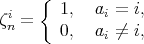
Consider the set of all permutations of
 ,
assigning the probability ,
assigning the probability  to each of them. For the permutation to each of them. For the permutation
 the number of its fixed points is defined as the number of indices
 such that such that
 . (In sorting, fixed points do not need to
be swapped transfered, which can be used in some forms of sorting.) Is it true that,
for a fixed . (In sorting, fixed points do not need to
be swapped transfered, which can be used in some forms of sorting.) Is it true that,
for a fixed  the expectation of the number of fixed points of the permutation is equal to:
|
|
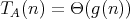
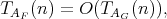
As was discussed above, the worst- and average-case complexities of an algorithm are both a function of a numerical argument-the input size. The growth of the complexity of a particular algorithm with increasing input size is frequently analyzed using asymptotic bounds of the form
 is on the order of is on the order of
 ”, or
“ ”, or
“ and and
 are of the same order”. are of the same order”.
|
|
|
|
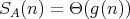
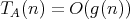
A comparison of the complexities of different algorithms based on their asymptotic
complexity bounds can be made not for all types of such bounds.
For example, if algorithms |
|
|
|
|
|
|
|
Question:
Suppose that the polynomial
 has a nonzero leading coefficient
  .
Which of the following assertions is true: .
Which of the following assertions is true:
|
|
Question:
Which of the following assertions is not true for the complexity
 of the trial division algorithm (see Section 1), which is intended for testing the primality of
an integer
of the trial division algorithm (see Section 1), which is intended for testing the primality of
an integer  (we mean the complexity measured as the number of divisions): (we mean the complexity measured as the number of divisions):
|
|
Question:
Let the cost of any compass-and-straightedge construction in plane geometry be the number of lines
(circles or straight lines) drawn in the course of the construction. Consider the problem of constructing
a line segment whose length is
 of that of the original segment, assuming that
  is the input size. Is there an algorithm for solving the problem whose complexity bound is
 ? ?
|
|
We can consider different complexities according to the costs taken into account. Suppose that a time cost function gives the number of operations of some type, assuming that they require an identical runtime independent of the operand size and set equal to 1. Then we obtain an algebraic complexity measured as the number of operations of the given type. |
|
|
|
Bit time complexity is obtained when the number of bit operations is used as a cost function. In a similar fashion, the space algebraic and bit space complexities can be defined using the number of operations values of the considered type. |
|
|
|
|
Question:
It is well known that the multiplicative complexity of Gaussian elimination as applied to a system of
 linear equations with linear equations with
 unknowns satisfies the bounds estimates unknowns satisfies the bounds estimates
|
|
Question:
Suppose that two positive integers
 and and
 are multiplied using the additions are multiplied using the additions
 and
and  (denoted by
  ).
Which of the following bounds is true for the complexity of this "supernaive" multiplication: ).
Which of the following bounds is true for the complexity of this "supernaive" multiplication:
|
|
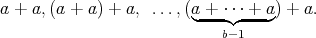
Question:
Given a number initially equal to zero, a 1 is added to it at every step until
 , ,
 , is reached. All the additions are performed in columns
in the binary system. Is it true that , is reached. All the additions are performed in columns
in the binary system. Is it true that  transfers of 1 to the next position on the left are required in these additions?
|
|
The concept of complexity is also considered in the case of randomized algorithms, i.e., algorithms making calls to a random number generator with a known distribution. |
|
|
|
Generally, the cost of a randomized algorithm is not uniquely determined by its input, but also depends on the generated random numbers. However, the averaged cost for each particular input gives a scalar numeric function on the set of inputs. As a result, the complexity of an algorithm can be treated following the general definition of complexity. |
|
|
|
|
As was previously discussed, the average-case complexity of a "usual" (deterministic) algorithm is of interest only if correct assumptions are made about the probability of occurrence of one or another input. The considered complexity of randomized algorithms is worst-case complexity but it is determined by the averaged costs. Nevertheless, this averaging can be trusted, since randomized algorithms make use of random number generators in which the probability distribution is fixed and independent of the inputs. |
|
|
|
|
|
Question:
Is it true that the determination of the averaged cost of a randomized algorithm requires specifying a probability distribution:
|
|
Question:
An array
 is said to contain a majority if more than half of its elements have identical values.
Let the operation of verifying whether two elements are equal be defined over the array
elements. This operation is called comparison. Given a majority-containing array, the goal
is to find an
is said to contain a majority if more than half of its elements have identical values.
Let the operation of verifying whether two elements are equal be defined over the array
elements. This operation is called comparison. Given a majority-containing array, the goal
is to find an  , ,
 , such that the value , such that the value
 belongs to the majority of values of
  .
A possible randomized algorithm for solving this problem is that .
A possible randomized algorithm for solving this problem is that
 is chosen at random (a uniform probability distribution) and
it is then verified whether
is chosen at random (a uniform probability distribution) and
it is then verified whether
 satisfies the above condition. The number of comparisons required for this verification is
 . If . If
 does not satisfy the condition, all
steps are repeated. Is it true that the complexity measured as the number of comparisons
in this randomized algorithm with does not satisfy the condition, all
steps are repeated. Is it true that the complexity measured as the number of comparisons
in this randomized algorithm with  taken as an input size is less than
  ? ?
|
|
Question:
Assume that there is a random number generator returning 0 with probability
 or 1 with probability
  ; moreover, it is
only know about ; moreover, it is
only know about  that that
 and
and  . This generator can be used to
design another one returning 0 or 1 with identical
probability . This generator can be used to
design another one returning 0 or 1 with identical
probability  :
generating two digits in succession with the help of the original generator, we obtain
the combinations 0, 1 and 1, 0 with an identical nonzero probability (the combinations
0, 0 and 1, 1 are ignored). Consider the expected number :
generating two digits in succession with the help of the original generator, we obtain
the combinations 0, 1 and 1, 0 with an identical nonzero probability (the combinations
0, 0 and 1, 1 are ignored). Consider the expected number
 of calls to the original random number generator
that are required in the construction of a sequence of pairs until 0, 1 or 1, 0 occur.
Which of the following assertions is true: of calls to the original random number generator
that are required in the construction of a sequence of pairs until 0, 1 or 1, 0 occur.
Which of the following assertions is true:
|
|
|
In computational complexity theory, initial assumptions are made about a hypothetical computing device (known as a model of computation). |
|
A random-access machine (RAM) is used as such a model in some cases, while a Turing machine is chosen in other cases. |
|
|
|
|
The former model is closer to actual devices, while the latter is more formalized, which is frequently useful in the existence analysis of an algorithm with certain complexity properties. |
|
|
We will use the RAM model. The assumption that the size of a cell is unlimited leads to algebraic complexity, while the assumption that one bit is stored in a cell leads to time or space bit complexity. |
|
The considered concept of complexity is sometimes referred to as computational complexity (its possible special cases are algebraic and bit complexities) in order to distinguish it from descriptive complexity, which is somehow defined relying on the code of an algorithm. |
|
|
|
|
Only computational complexity is discussed below, and we continue to refer to it as complexity. |
|
Considering a class of algorithms for solving a problem yields a family of functions that are complexities (for example, time complexities) of algorithms in this class. Accordingly, we can discuss a lower bound for this family and the existence of a minimal function in it. |
|
|
|
If there is a minimal function in this family, then the corresponding algorithm is optimal in the considered class of algorithms. |
|
|
|
|
Question:
Is
 an asymptotic lower bound for the complexity of algorithms for
compass-and-straightedge division of a segment into
an asymptotic lower bound for the complexity of algorithms for
compass-and-straightedge division of a segment into
 equal parts
with equal parts
with  regarded as an input size (the cost of any compass-and-straightedge
construction in the plane is assumed to be the number of lines
(circles or straight lines) drawn in the course of the construction)?
regarded as an input size (the cost of any compass-and-straightedge
construction in the plane is assumed to be the number of lines
(circles or straight lines) drawn in the course of the construction)?
|
|
Question:
Consider the problem of computing
 in a set with associative multiplication (i.e., in a semigroup), where
 is a given positive integer regarded as an input size. Is
 an asymptotic lower bound for the complexity of algorithms for computing
 with the help of multiplications?
|
|
Question:
A traveler encounters a wall that extends to infinity in both directions.
There is a door in the wall, but neither the distance to it nor
the direction toward it is known to the traveler. Let the input size be the number
 of steps
(unknown to the traveler) that initially separate the traveler from the door. Clearly, of steps
(unknown to the traveler) that initially separate the traveler from the door. Clearly,
 is a lower and an asymptotic lower bound for door-reaching algorithms
(in all cases, the traveler has to take
is a lower and an asymptotic lower bound for door-reaching algorithms
(in all cases, the traveler has to take  steps). Can a door-reaching algorithm with
 complexity bound be proposed? complexity bound be proposed?
|
|
Question:
Is it true that the function
 is a lower complexity bound for algorithms intended for simultaneously selecting
the largest and smallest maximal and minimal elements in an array of
length
is a lower complexity bound for algorithms intended for simultaneously selecting
the largest and smallest maximal and minimal elements in an array of
length  with the help of comparisons?
|
|
Question:
Let
 be a comparison sort algorithm and be a comparison sort algorithm and
 denote the number of elements in the input array. Let denote the number of elements in the input array. Let
 , ,  -
be the complexities of -
be the complexities of  measured as the number of
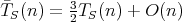
comparisons in the worst and average cases, respectively. Which of the following equalities does not hold for any measured as the number of
comparisons in the worst and average cases, respectively. Which of the following equalities does not hold for any
 : :
|
|
Optimal algorithms in a given class are not always known. It is also possible that a given class has no optimal algorithm, i.e., an algorithm whose complexity is a lower complexity bound for algorithms in this class. |
|
|
|
Rather frequently, it is very difficult to answer whether a particular class of algorithms has one whose complexity does not grow too fast with increasing input size. |
|
|
|
For some classes of algorithms, a difficult question is whether there exists an algorithm in such a class with complexity bounded above by a polynomial whose form is not specified (such an algorithm is known as polynomial-time). |
|
|
|
In particular, many unanswered questions concern polynomial-time algorithms for decision problems, i.e., those having a yes/no solution, or a 1/0 solution, etc. In this context, we mention the well-known P≟NP problem. |
|
|
|
|
Question:
Assume that the cost of any compass-and-straightedge construction in the plane is the number of lines
(circles or straight lines) drawn in the course of the construction. Consider the problem
of constructing a segment whose length is
 of that of the original segment, assuming that of that of the original segment, assuming that
 is the input size. Is there a solution algorithm whose complexity grows more
slowly than
is the input size. Is there a solution algorithm whose complexity grows more
slowly than  ? ?
|
|
Question:
The existence of a polynomial-time algorithm for decomposing an integer
 of bit length
  into prime factors remains
an open problem, although factorization algorithms are of great importance in cryptography.
In this context, consider the following problem: given into prime factors remains
an open problem, although factorization algorithms are of great importance in cryptography.
In this context, consider the following problem: given  , ,
 , determine whether , determine whether
 has a divisor
  such that such that
 . No polynomial-time algorithm (in terms of the bit length of . No polynomial-time algorithm (in terms of the bit length of
 of of  )
is available for this problem. Is it true that, if such an algorithm )
is available for this problem. Is it true that, if such an algorithm  were devised, this would automatically produce a polynomial-time factorization algorithm?
|
|
Question:
Is it possible to compute the product of two given complex numbers
 using several additions and subtractions and only three multiplications of real numbers?
(Assume that the values
using several additions and subtractions and only three multiplications of real numbers?
(Assume that the values  , ,
 have been computed;
how can a suitable number have been computed;
how can a suitable number  be
found using a single multiplication so that the computation of the required quantities
can be completed using only additions and subtractions?) be
found using a single multiplication so that the computation of the required quantities
can be completed using only additions and subtractions?)
|
|
Question:
Is it true that P
 NP
will be proved if we show that at least one problem in NP is in P? NP
will be proved if we show that at least one problem in NP is in P?
|
|
|
When we examine the existence of an algorithm of "not very high" complexity, an important role is played by the reducibility of one problem to another. The possibility of quickly solving some problem can imply the same possibility for a number of other problems and, on the contrary, if a certain problem cannot be quickly solved, the same can automatically be implied for a number of other problems. |
|
Considering linear reducibility, we can rigorously define the fact that one computational problem is not harder than another. |
|
|
|
Polynomial reducibility means that, if a computational problem is solvable by a polynomial-time algorithm, then another problem is also solvable by a polynomial-time algorithm. |
|
|
|
|
Question:
Is the multiplication of arbitrary square matrices linearly
reducible (see above in this section) to the multiplication of upper
triangular matrices, assuming that the latter problem is solved only by algorithms
for which
 (as occurs for all reasonable algorithms designed for this problem)?
|
|
Question:
Are there problems in NP that are not NP-complete?
|
|
Question:
Imagining that there is no polynomial-time algorithm for testing
the primality of a positive integer (i.e., the AKS algorithm (see Section 9) does not exist),
would it be true that P
 NP? NP?
|
|
Along with various questions concerning the possible limits for algorithms from one or another class, always important are problems associated with complexity bounds for particular algorithms. Frequently, trivial upper and lower bounds are easy to derive, while deriving close-to-tight bounds for an algorithm requires much effort and nontrivial approaches. |
|
|
|
|
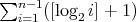
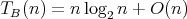
Question:
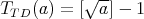
A binary algorithm for finding an element place in an ordered array of length
 has complexity
  , which implies
that the complexity , which implies
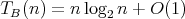
that the complexity  of binary insertion sort is
 . The last
term in this sum is the largest, which yields . The last
term in this sum is the largest, which yields
 .
Is it true that .
Is it true that 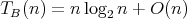 ? ?
|
|
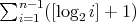
Question:
The complexity
 measured as the number of comparisons in binary insertion sort is
 .
For some values of .
For some values of  , ,
 elements can be sorted using a smaller number of comparisons. Which is the smallest
 of this kind:
|
|
Question:
Is it true that
 for the complexity
  measured as the number of comparisons in the binary insertion sort as applied to an array of
 elements? (Recall that this complexity is equal to
 .) .)
|
|
Question:
Let
 be the average number of assignments
  executed in the following algorithm for finding the smallest element of an array
for
if od assuming that all possible relative orders of the elements in the original array of length are equiprobable. Which of the following assertions is true:
|
 is considered from the point of view of complexity, it is assumed that, at its possible inputs
 , we are given the nonnegative integer function
 ,
which is known as the input size,
and nonnegative integer time and space cost functions
,
which is known as the input size,
and nonnegative integer time and space cost functions
 ,
,
 (space cost is also known as memory storage cost; the cost required for storing the input itself is ignored).
 are
functions of numerical argument defined as
are
functions of numerical argument defined as

 are functions of numerical argument defined as

 regarded as an argument of
  and
and
 is the range of the size
 ).
).
 of some length
  .
The number of comparisons required by this algorithm for fixed
.
The number of comparisons required by this algorithm for fixed
 , ranges from
 to
to
 . Therefore, if
 is taken as the input size, the complexity
 of the algorithm is
  comparisons. The complexity
 measured as the number of swaps
(
measured as the number of swaps
( ) is equal to the same function of
 . The space complexity
 is bounded by a small constant (the original array is replaced by an ordered array).
 . If
. If
 is taken as the input size, then the time complexity of this algorithm is
 , multiplications, while the space complexity is
 (the product is computed in a new place).
 ,
is prime, which is referred to as the trial division algorithm, determines whether there is at least one integer between
1 and
,
is prime, which is referred to as the trial division algorithm, determines whether there is at least one integer between
1 and  ,
that divides
,
that divides  .
The number of checks whether
.
The number of checks whether  is divided by one or another integer (for brevity, the "number of divisions") ranges from
 to
to  (here
(here
 — denotes the integer part of a number). Denoting this
algorithm by TD (from trial divisions) and assuming that the input size is
— denotes the integer part of a number). Denoting this
algorithm by TD (from trial divisions) and assuming that the input size is
 itself, we can say that for any
  the value of
  is at most
  ,
and there are arbitrarily large
,
and there are arbitrarily large  ,
for which this value is equal to
,
for which this value is equal to  .
Obviously, the values of
.
Obviously, the values of  are bounded by a small constant.
 can be considerably larger or smaller than its output size.
 does not imply that
  is always less than
 .
.
 .
.
 , the corresponding inputs form a finite set
 .
Assume that each
.
Assume that each  is assigned some probability
  :
:
 and
and
 . Thus, the time and space cost functions
 and
and  of an algorithm
 on inputs
 of size
  are random variables on
  .
The average-case time and space complexities of
.
The average-case time and space complexities of 
 ,
the corresponding inputs form a finite set
,
the corresponding inputs form a finite set
 .
Assume that each
.
Assume that each  is assigned some probability
  :
:
 and
and
 .
Thus, the time and space cost functions
.
Thus, the time and space cost functions
 and
and
 of an algorithm
 on inputs
 of size
 are random variables on
 . The average-case time and space complexities
of
. The average-case time and space complexities
of 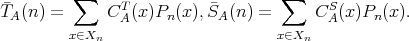
 ; the only
important point is their relative order. Therefore, we can assume that the arrays of
length
; the only
important point is their relative order. Therefore, we can assume that the arrays of
length  ,
to which sorting algorithms are applied are the permutations of the numbers
,
to which sorting algorithms are applied are the permutations of the numbers
 . For each
 we can consider the set of permutations of
 , assigning the probability
 to each of them.
As a result, the average-case complexity of sorting algorithms can be considered.
It can be proved that the complexity
to each of them.
As a result, the average-case complexity of sorting algorithms can be considered.
It can be proved that the complexity
 of the quicksort algorithm QS measured as the number of comparisons satisfies
 . The average-case complexity of
quicksort measured as the number of transfers is at most
. The average-case complexity of
quicksort measured as the number of transfers is at most
 ,
where
,
where  is a small constant. The space complexity
is bounded by a constant. (Additionally, a stack of suspended postponed tasks is used, which contains
element indices rather than the elements themselves.)
is a small constant. The space complexity
is bounded by a constant. (Additionally, a stack of suspended postponed tasks is used, which contains
element indices rather than the elements themselves.)
 for any probability distribution on the set
 , the average-case complexity
does not exceed the worst-case complexity:
, the average-case complexity
does not exceed the worst-case complexity:
 ,
,
 .
.
 for any probability distribution on the set
 , the average-case complexity
does not exceed the worst-case complexity:
, the average-case complexity
does not exceed the worst-case complexity:
 ,
,
 .
.
 , the worst-case complexity
of quicksort measured as the number of comparisons grows as
, the worst-case complexity
of quicksort measured as the number of comparisons grows as
 ,
while the average-case complexity is at most
,
while the average-case complexity is at most
 (see the above argument in this section).


 . It can be seen that
 , whence
 and, as a consequence, the expectation
of interest is
and, as a consequence, the expectation
of interest is


 holds if and only if there are positive
 such that
 for all
  .
.
 and
and  are of the same order (written as
 )
if and only if there are positive
)
if and only if there are positive
 such that

 .
.

 .
Additionally, we can show that
.
Additionally, we can show that
 and
and  : a consequence of
Stirling's formula is the bound
: a consequence of
Stirling's formula is the bound
 does not imply that
  .
For example
.
For example  , but it is not true that
 .
.
 and
and
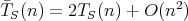
 have respective complexities
 such that
 ,
,
 , it cannot be concluded that
 for all sufficiently large
  .
.
 and
and  do not imply that
 , the relations
 ,
,
 do not imply that
 for all sufficiently large
  .
.
 (or
(or  ) is suitable for
"praising" an algorithm
) is suitable for
"praising" an algorithm  ,
i.e., for characterizing its complexity as rather low, but not for "criticizing" it-for this goal, a bound of the form
,
i.e., for characterizing its complexity as rather low, but not for "criticizing" it-for this goal, a bound of the form
 is more appropriate.
 ,
,
 , which combine the bounds
 and
and 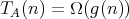 , or
, or
 and
and  ,
are suitable for characterizing both relatively low and relatively high complexities
in corresponding situations.
,
are suitable for characterizing both relatively low and relatively high complexities
in corresponding situations.
 ,
,
 ,
,
 ?
?
 also holds for
  .
Assertion 2 is not true, since
.
Assertion 2 is not true, since
 also holds for
  .
Assertion 3 is true, since both
.
Assertion 3 is true, since both
 and
and  hold only for
  .
.
 ,
,
 ,
,
 ,
,
 ?
?
 .
Therefore, 1 and 4 are true. For
.
Therefore, 1 and 4 are true. For  at least one division is required; therefore, 2 is true. If 3 were true, we would have
 ,
which does not hold, since
,
which does not hold, since
 for an infinite set of values of
 .
.
 times as long, both starting from the vertex. The latter can be done with
 cost by doubling and adding segments
(preliminarily, it is convenient to represent
cost by doubling and adding segments
(preliminarily, it is convenient to represent
 in the binary number system). By the Thales intercept theorem, the construction
is completed with
in the binary number system). By the Thales intercept theorem, the construction
is completed with  cost. The total cost is
 , which is uniquely determined by
the input size. Therefore, the complexity of the algorithm is
, which is uniquely determined by
the input size. Therefore, the complexity of the algorithm is
 .
.
 (worst-case complexities are meant).
 and
and  , are multiplied, the multiplicative complexity is
1 regardless of the input size. However, for long multiplication with input
size
, are multiplied, the multiplicative complexity is
1 regardless of the input size. However, for long multiplication with input
size  - the bit length
(the number of digits in the binary representation) of the larger number,
the worst-case bit time complexity is
- the bit length
(the number of digits in the binary representation) of the larger number,
the worst-case bit time complexity is  .
.
 bit) complexity.
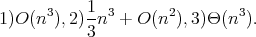
 follows from any of 1), 2), 3).
 does not follow from (1), which is an upper bound, while
 is a lower bound.
 ,
,
 ,
,
 ?
?
 and
and  have an identical bit length, each addition requires at least
 bit operations; moreover
 , which yields
 for the complexity under study.
On the other hand,
for the complexity under study.
On the other hand,  .
Therefore, the result of each step has a bit length of at most
.
Therefore, the result of each step has a bit length of at most
 . This means that the number of bit operations
at each step is at most
. This means that the number of bit operations
at each step is at most
 , where
  is a constant. This yields
  ,
and, finally, the bound
,
and, finally, the bound  .
.
 denotes the number of transfers of 1 and the quantity
 has been obtained by adding 1's (which requires
 transfers), then the next addition of 1 requires
 transfers and yields the quantity
  ,
whose binary representation is
,
whose binary representation is  (the number of 0's following 1 is
  ).
To reach
).
To reach  (
( 1's) another
 transfers are required.
 of positive integer argument
  ,
that returns one of the elements of the set
,
that returns one of the elements of the set
 ,
so that the value of this function cannot be reliably predicted - any element of the above
set can appear with probability
,
so that the value of this function cannot be reliably predicted - any element of the above
set can appear with probability  .
.
 complexity measured as the number of comparisons assuming that all the relative orders
of the elements in the original array are equiprobable (see Section 2). In some situations,
this assumption can be groundless; for example, the array can be almost ordered by construction.
However, if the partitioning elements at all the stages of the partition operation are chosen at
random with a corresponding probability, then this randomized quicksort algorithm has
complexity measured as the number of comparisons assuming that all the relative orders
of the elements in the original array are equiprobable (see Section 2). In some situations,
this assumption can be groundless; for example, the array can be almost ordered by construction.
However, if the partitioning elements at all the stages of the partition operation are chosen at
random with a corresponding probability, then this randomized quicksort algorithm has
 complexity without assuming
the equiprobability of all the relative orders of the elements.
complexity without assuming
the equiprobability of all the relative orders of the elements.
 with an input
  one needs the probabilities of the scenarios assigned by
 to
to  . Then the computational
cost for each such scenario defines a random variable on the probability
space of scenarios assigned to
. Then the computational
cost for each such scenario defines a random variable on the probability
space of scenarios assigned to
 .
Its expectation is the value of the averaged cost function for
.
Its expectation is the value of the averaged cost function for
 .
.
 the set of all possible scenarios is the set of tuples of the form
 , where
 and all
 are the integers from
 to
to  ,
moreover
,
moreover  do not belong to the majority, while
  does. In a natural manner, these scenarios can be assigned probabilities. The space of
scenarios is decomposed into two events: the first attempt to find
the required
does. In a natural manner, these scenarios can be assigned probabilities. The space of
scenarios is decomposed into two events: the first attempt to find
the required  is successful and unsuccessful, respectively. Let
 ,
where
,
where  is the number of elements of
the majority in the given array (input). By assumption
is the number of elements of
the majority in the given array (input). By assumption
 .
The averaged cost
.
The averaged cost  satisfies the equality
  .
We obtain
.
We obtain  .
Thus, for any input of size
.
Thus, for any input of size  the averaged cost is less than
  .
Therefore, the complexity of the algorithm is less than
.
Therefore, the complexity of the algorithm is less than  and, hence, less than
  .
.
 reaches its minimum at
 ,
,
 reaches its minimum at
 ,
,
 the values of
  decrease monotonically,
 is independent of
  ?
?
 .
.
 be a fixed class of algorithms
for solving some problem. Suppose that the cost of an algorithm and
the size of its input have been defined. Let
be a fixed class of algorithms
for solving some problem. Suppose that the cost of an algorithm and
the size of its input have been defined. Let
 denote the input size. A function
 is said to be a lower bound for the complexity of algorithms in
 if the complexity
 of any
  satisfies
 for all
admissible input sizes
for all
admissible input sizes  .
.
 be a fixed class
of algorithms for solving some problem. Suppose that the cost of an algorithm
and the size of its input have been defined.
Let
be a fixed class
of algorithms for solving some problem. Suppose that the cost of an algorithm
and the size of its input have been defined.
Let  denote the input size. A function
  is said to be a lower bound for the complexity of algorithms in
 if the complexity
 of any
 satisfies
 for all admissible input sizes
 .
.
 is a lower complexity bound for algorithms of comparison-based search for the least minimal
element in a numerical array of length
is a lower complexity bound for algorithms of comparison-based search for the least minimal
element in a numerical array of length  .
Indeed, for an array element to be eliminated as inappropriate, it has to be compared at least
once and be found larger than its contender. We need to eliminate
.
Indeed, for an array element to be eliminated as inappropriate, it has to be compared at least
once and be found larger than its contender. We need to eliminate
 elements and, in each comparison, precisely one element is larger than another. This
means that at least
elements and, in each comparison, precisely one element is larger than another. This
means that at least  comparisons are required.
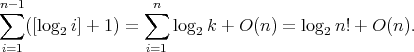
 is a lower complexity bound in the worst and average cases for comparison sort algorithms
applied to arrays consisting of
is a lower complexity bound in the worst and average cases for comparison sort algorithms
applied to arrays consisting of  pairwise distinct numbers (in the average case, all the relative orders of the elements
in the original array are assumed to have identical probability
pairwise distinct numbers (in the average case, all the relative orders of the elements
in the original array are assumed to have identical probability
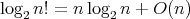
 ). In the context of the last example,
we note that Stirling's formula implies
). In the context of the last example,
we note that Stirling's formula implies
 .
.
 such that
  for some lower complexity bound
  then
then  is called asymptotically optimal, or optimal in the order
of complexity.
is called asymptotically optimal, or optimal in the order
of complexity.
 comparisons is optimal in the class of algorithms for finding the least
element in a numerical array of length
comparisons is optimal in the class of algorithms for finding the least
element in a numerical array of length
 .
All comparison sort algorithms for arrays consisting of
.
All comparison sort algorithms for arrays consisting of
 pairwise distinct numbers that have
 complexity measured as the number of comparisons are optimal in the order of
complexity, and their complexity is
complexity measured as the number of comparisons are optimal in the order of
complexity, and their complexity is
 .
.
 is said to be an asymptotic lower
bound for the complexity of algorithms in
is said to be an asymptotic lower
bound for the complexity of algorithms in
 if the complexity
  of any
 satisfies
 .
Any lower bound is an asymptotic lower bound as well, but the converse is
generally not true. It is easy to show that, if an algorithm
.
Any lower bound is an asymptotic lower bound as well, but the converse is
generally not true. It is easy to show that, if an algorithm
 is asymptotically
optimal in the class
is asymptotically
optimal in the class
 , then its complexity is
an asymptotic lower bound for the complexity of algorithms in
, then its complexity is
an asymptotic lower bound for the complexity of algorithms in
 .
.
 points. Each operation (of drawing a circle or straight line) yields at most two points on
the segment: a circle intersects the segment in at most two points, while a straight line,
in at most one point. Therefore,
points. Each operation (of drawing a circle or straight line) yields at most two points on
the segment: a circle intersects the segment in at most two points, while a straight line,
in at most one point. Therefore,  is a lower complexity bound for the considered algorithms. Consequently,
 is an asymptotic lower bound.
 to the
  th power is that if the binary representation of
 is
is  , then the computation of
 can be reduced to computing the sequence of values
 (each element of the sequence is obtained by squaring the previous one) and to computing
the product
(each element of the sequence is obtained by squaring the previous one) and to computing
the product  of those
  for which
 .
The complexity of this algorithm is at most
.
The complexity of this algorithm is at most  .
It can be shown that
.
It can be shown that  is a lower complexity bound for all algorithms of this form; see, for example,
 then
then
 can be raised to the
 th power with a smaller number
of multiplications than required by the binary algorithm.
th power with a smaller number
of multiplications than required by the binary algorithm.
 bound, it is sufficient to note that
  is a quantity of order
  ,
i.e.
,
i.e.  , and, in the case under study,
 is such that
 .
.
 comparisons. The elements
  of the array are searched through in consecutive pairs:
 , then
 etc. (the last element may remain without a pair). In the
 th pair
 the smaller and larger elements are compared with the smallest and largest elements
found previously among
the smaller and larger elements are compared with the smallest and largest elements
found previously among  .
If
.
If  is odd, then, at the last step,
  is compared with the smallest and largest elements found among
 .
Additionally, the function
.
Additionally, the function  is a lower complexity bound for comparison-based algorithms designed for simultaneously selecting
the largest and smallest elements in an array of length
is a lower complexity bound for comparison-based algorithms designed for simultaneously selecting
the largest and smallest elements in an array of length
 :
:
 ,
,
 ?
?
 is a lower complexity bound for sorting algorithms in both worst and average cases.
We have
is a lower complexity bound for sorting algorithms in both worst and average cases.
We have  .
Moreover,
.
Moreover, 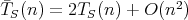 holds for any sort whose worst-case complexity is
 .
.
 ,
as input, which is also its size. Let the complexity of one algorithm be low for
even
,
as input, which is also its size. Let the complexity of one algorithm be low for
even  ,
and high for odd and vice verse for the other algorithm. The arising family of
two functions has no minimal one. Accordingly, there is no optimal
algorithm in the considered class.
,
and high for odd and vice verse for the other algorithm. The arising family of
two functions has no minimal one. Accordingly, there is no optimal
algorithm in the considered class.
 , where
 is the bit length (the number of digits
in the binary representation) of the larger of two numbers to be multiplied. In 1962
A.A. Karatsuba found an algorithm of
is the bit length (the number of digits
in the binary representation) of the larger of two numbers to be multiplied. In 1962
A.A. Karatsuba found an algorithm of  complexity (here,
  ).
In 1963, generalizing Karatsuba's idea and invoking interpolation, A.L. Toom showed that for every
).
In 1963, generalizing Karatsuba's idea and invoking interpolation, A.L. Toom showed that for every
 there exists a multiplication algorithm of
 ;
complexity. More specifically, for any integer
;
complexity. More specifically, for any integer  there exists a multiplication algorithm of complexity
 , where
 .
In 1972 A. Schönhage and V. Strassen used a special form of interpolation - fast Fourier transform -
to design an algorithm of complexity
.
In 1972 A. Schönhage and V. Strassen used a special form of interpolation - fast Fourier transform -
to design an algorithm of complexity
 .
If
.
If  in this algorithm has the form of
 ,
then
,
then  in the complexity bound can be replaced by
 . Finally, in 2007 M. Fürer proposed an algorithm
of complexity
. Finally, in 2007 M. Fürer proposed an algorithm
of complexity  , where
 is a function growing more slowly than
 and even more slowly than any iterated logarithm. It is unclear how much this result can be
further improved in this direction, in particular, whether a multiplication algorithm of complexity
and even more slowly than any iterated logarithm. It is unclear how much this result can be
further improved in this direction, in particular, whether a multiplication algorithm of complexity
 exists.
 exists.
 is
is  ,
arithmetic operations, while the algorithm following directly from
the definition of matrix product has
,
arithmetic operations, while the algorithm following directly from
the definition of matrix product has
 complexity (here,
 ).
Relying on other ideas, in 1987 D. Coppersmith and S. Winograd proposed
an algorithm with
).
Relying on other ideas, in 1987 D. Coppersmith and S. Winograd proposed
an algorithm with
 arithmetic operations,
where
arithmetic operations,
where  is the order of the square matrices to be multiplied. In 2012 V. Vassilevska Williams
published an algorithm which has O(n^{2.3727}) complexity measured as the number of arithmetic operation.
This result has remained the best to this day. Whether for any
is the order of the square matrices to be multiplied. In 2012 V. Vassilevska Williams
published an algorithm which has O(n^{2.3727}) complexity measured as the number of arithmetic operation.
This result has remained the best to this day. Whether for any  there is an
 time algorithm for matrix multiplication remains an open question.
 is the size of the input, then an
algorithm is polynomial-time if and only if its complexity is
is the size of the input, then an
algorithm is polynomial-time if and only if its complexity is
 for some
  .
.
 ,
bit complexity, where the input size is the bit length
,
bit complexity, where the input size is the bit length
 of the input number; the algorithm was published by M. Agrawal, N. Kayal, and N. Saxena in
2004 and is referred to as AKS algorithm.
(For this input size, the complexity of the trivial TD algorithm (see Section 1) measured
as the number of divisions (not bit operations) is
of the input number; the algorithm was published by M. Agrawal, N. Kayal, and N. Saxena in
2004 and is referred to as AKS algorithm.
(For this input size, the complexity of the trivial TD algorithm (see Section 1) measured
as the number of divisions (not bit operations) is
 .)
.)
 ,
represented like the original object
,
represented like the original object  ,
by a finite sequence of symbols, i.e., by a string word over some alphabet
,
by a finite sequence of symbols, i.e., by a string word over some alphabet
 .
The lengths of the strings
.
The lengths of the strings  and
and  are denoted by
 and
and  . The size of the input
 is
is
 ; the time cost is measured as
the number of operations with symbols (by analogy with bit operations). We specify
a polynomial
; the time cost is measured as
the number of operations with symbols (by analogy with bit operations). We specify
a polynomial  and a two-place predicate
  ,
defined on strings over
,
defined on strings over  .
The predicate has the property that, for strings
.
The predicate has the property that, for strings
 such that
 , the time required for computing
 is bounded above by a polynomial in
 .
The corresponding problem in NP is to answer whether it is true that
.
The corresponding problem in NP is to answer whether it is true that

 .
(For most problems in NP, it holds that
.
(For most problems in NP, it holds that
 i.e., the string
 is not longer than
 .)
.)
 ,
and nonempty strings be interpreted as binary nonnegative integers.
Then the verification of whether a given number
,
and nonempty strings be interpreted as binary nonnegative integers.
Then the verification of whether a given number
 is composite can be stated
as a problem in NP: here, the predicate (condition)
is composite can be stated
as a problem in NP: here, the predicate (condition)
 is
is
 and
and  is divided by
 ”,
”,
 . The verification of whether
 is divided by
 takes
takes
 time, where
 is the bit length of
  , i.e., the length of
 as a string over the alphabet
 .
.
 such that its value
 can be computed by a polynomial-time algorithm. It is easy to see that
P
can be computed by a polynomial-time algorithm. It is easy to see that
P NP:
for example, we can use
NP:
for example, we can use  ,
,
 .
.
 defines a one-place predicate
  .
It is not always clear whether there is a polynomial-time algorithm for computing the value of
.
It is not always clear whether there is a polynomial-time algorithm for computing the value of
 .
.
 determine whether there is an
assignment to the variables that makes the formula evaluate to TRUE.
determine whether there is an
assignment to the variables that makes the formula evaluate to TRUE.
 of the same commensurate length as a given string
 ,
we can quickly verify whether
,
we can quickly verify whether  and
and
 satisfy some fixed conditions, then we can
quickly verify whether there is at least one string
satisfy some fixed conditions, then we can
quickly verify whether there is at least one string  of the corresponding length that, together with
  ,
satisfies these conditions.
,
satisfies these conditions.
 NP conjecture).
 ) holds for a given
 : it is possible to search through all strings
 such that
 , each time verifying the condition
 .
However, the complexity of this algorithm grows exponentially as
.
However, the complexity of this algorithm grows exponentially as  .
.
 be used as a unit one. It is sufficient if we can quickly construct
a segment of length
be used as a unit one. It is sufficient if we can quickly construct
a segment of length
 ; this operation
will be referred to as "the construction of
the number
; this operation
will be referred to as "the construction of
the number  ."
Then the main problem can be solved by applying the Thales intercept theorem.
The following three facts are used here:
."
Then the main problem can be solved by applying the Thales intercept theorem.
The following three facts are used here:
 complexity (the construction of the product is based on the geometric
mean theorem, which describes the length of the altitude dropped to
the hypotenuse in a right triangle; this theorem is applied twice).
complexity (the construction of the product is based on the geometric
mean theorem, which describes the length of the altitude dropped to
the hypotenuse in a right triangle; this theorem is applied twice).
 can be written in the factorial number system:

 , where
 is the inverse of the gamma function.
 :
:
 are sequentially
constructed. This requires
are sequentially
constructed. This requires  additions.
 are sequentially constructed.
This requires
are sequentially constructed.
This requires  multiplications.
 is constructed using the numbers obtained.
This requires
is constructed using the numbers obtained.
This requires  additions and the same number of multiplications.
 complexity.
It was proposed in the paper
complexity.
It was proposed in the paper
 ,
the prime factors of
,
the prime factors of  can be found via binary search. Assume that it is known that
 has no divisors smaller than
 , where
 , and let
 be such that
 .
We are interested in the smallest prime factor of
.
We are interested in the smallest prime factor of
 lying between
 and
and  . By applying
 to
to
 , where
 ,
the range of the search is roughly halved. Initially, we set
,
the range of the search is roughly halved. Initially, we set
 .
Applying the algorithm
.
Applying the algorithm  at most
  times yields the smallest prime factor
 of
of
 . Similar computations are performed for
 etc. The total number of prime factors of
  counting multiplicity, is bounded above by
 , and, hence, by
 . The bit cost of each division is at most
 , where
 is a constant. If the bit complexity of
 is
is  ,
then the complexity of the prime factorization algorithm described is
,
then the complexity of the prime factorization algorithm described is
 ,
i.e., it is a polynomial-time algorithm.
,
i.e., it is a polynomial-time algorithm.
 ,
,
 ,
,
 .
.
 and
and
 be two computational problems. If any algorithm
 for solving
 can be put in correspondence with an algorithm
 for solving
 such that
 is said to be linearly reducible to
 . Alternatively,
 is said to be
not harder than
is said to be
not harder than  .
Here, "linearly" means only that the complexity of
.
Here, "linearly" means only that the complexity of
 is not, say, the square, cube, etc., of the complexity of
 .
.
 , to the inversion of
a matrix of order
, to the inversion of
a matrix of order
 (complexity measured as the number of arithmetic operations with matrix elements).
It can also be proved that, given a directed graph on
(complexity measured as the number of arithmetic operations with matrix elements).
It can also be proved that, given a directed graph on
 vertices without multiple edges that is represented by
its Boolean adjacency matrix, the construction of its transitive-reflexive closure
is linearly reducible to the multiplication of two
Boolean matrices of order
vertices without multiple edges that is represented by
its Boolean adjacency matrix, the construction of its transitive-reflexive closure
is linearly reducible to the multiplication of two
Boolean matrices of order  and
vice versa (bit complexity). In other words, progress achieved in the ability to
quickly solve one problem means the same progress for the other problem.
and
vice versa (bit complexity). In other words, progress achieved in the ability to
quickly solve one problem means the same progress for the other problem.
 to a problem
 means that, if
 solvable by a polynomial-time algorithm, then
 is also solvable by a polynomial-time algorithm. A problem
 is polynomially reducible to
 if any algorithm for
  can be applied to
  after quick (polynomially bounded in time) transformations of the input.
It is easy to show that the polynomial reducibility relation is transitive.
after quick (polynomially bounded in time) transformations of the input.
It is easy to show that the polynomial reducibility relation is transitive.
 NP (since any
NP-complete problem is in NP).
NP (since any
NP-complete problem is in NP).
 NP, then
 is also NP-complete,
which follows from the transitivity of polynomial reducibility.
is also NP-complete,
which follows from the transitivity of polynomial reducibility.
 are the original matrices of order
  .
.
 be positive integers such that
 .
The search for the greatest common divisor (GCD) of
.
The search for the greatest common divisor (GCD) of
 based on the Euclidean algorithm requires the execution of a series of
similar steps, each being division with a remainder:
based on the Euclidean algorithm requires the execution of a series of
similar steps, each being division with a remainder:
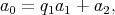


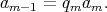
 GCD
GCD . The sequence of
obtained remainders decreases (a remainder is less than the corresponding divisor);
moreover, all the remainders are nonnegative integers. Therefore, the number of
divisions with a remainder is at most
. The sequence of
obtained remainders decreases (a remainder is less than the corresponding divisor);
moreover, all the remainders are nonnegative integers. Therefore, the number of
divisions with a remainder is at most  .
However, this easy-to-derive upper bound for the number of divisions with a remainder does
not reflect the basic advantages of the Euclidean algorithm. It turns out that the number of
divisions with a remainder is bounded by the logarithm of
.
However, this easy-to-derive upper bound for the number of divisions with a remainder does
not reflect the basic advantages of the Euclidean algorithm. It turns out that the number of
divisions with a remainder is bounded by the logarithm of
 .
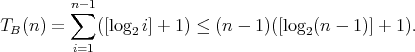
More specifically, it can be shown that, if
.
More specifically, it can be shown that, if
 is used as an input size, then the worst-case number of divisions required
in the Euclidean algorithm is
is used as an input size, then the worst-case number of divisions required
in the Euclidean algorithm is
 . Another surprise presented by
this algorithm is associated with its bit complexity. Let the input size be the bit length
. Another surprise presented by
this algorithm is associated with its bit complexity. Let the input size be the bit length
 (the number of digits in the binary representation)
of
(the number of digits in the binary representation)
of  . By what was said above, the worst-case
number of divisions with a remainder is
. By what was said above, the worst-case
number of divisions with a remainder is  .
For the naive division of two integers with a remainder, assuming that the bit length of the larger number is
.
For the naive division of two integers with a remainder, assuming that the bit length of the larger number is
 ,
the bit complexity is on the order of
,
the bit complexity is on the order of  , which easily
yields
, which easily
yields  for the bit complexity of the Euclidean algorithm. However, a more careful analysis shows
that the bit complexity of the Euclidean algorithm is
for the bit complexity of the Euclidean algorithm. However, a more careful analysis shows
that the bit complexity of the Euclidean algorithm is
 .
Additionally, it can be shown that this complexity cannot be significantly reduced
by applying "faster" forms of division: it still satisfies the bound
.
Additionally, it can be shown that this complexity cannot be significantly reduced
by applying "faster" forms of division: it still satisfies the bound
 for any division algorithm of complexity
 .
.
 , whence
 .
.
 this algorithm requires three and five comparisons, respectively. Since
 is a lower complexity
bound for sorting (see Section 8), the number of comparisons cannot be reduced
in this case. However, for
is a lower complexity
bound for sorting (see Section 8), the number of comparisons cannot be reduced
in this case. However, for
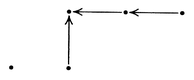
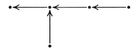
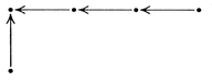
 this algorithm requires
eight comparisons; moreover, it is possible that five elements are to be sorted,
in which case only seven comparisons are required in the worst case. The algorithm
can easily be sketched by showing the compared elements by circles joined by an arrow
directed from larger to smaller elements. The first element is compared with the second,
the third element is compared with the fourth, and the smaller elements found in each case
are compared with each other. This requires three comparisons:
this algorithm requires
eight comparisons; moreover, it is possible that five elements are to be sorted,
in which case only seven comparisons are required in the worst case. The algorithm
can easily be sketched by showing the compared elements by circles joined by an arrow
directed from larger to smaller elements. The first element is compared with the second,
the third element is compared with the fourth, and the smaller elements found in each case
are compared with each other. This requires three comparisons:
 is an integer and
  it holds that
  .
Thus,
.
Thus,  for
for  ,
,


 to
to  do
do
 then
then  fi
fi
 ,
,
 ,
,
 ,
,
 ?
?
 ,
each assigned the probability
,
each assigned the probability  .
Consider the decomposition of this space into the sum of two events: the last element of
the original array is its smallest element
(with probability
.
Consider the decomposition of this space into the sum of two events: the last element of
the original array is its smallest element
(with probability  )
and the last element is not its smallest element (with probability
)
and the last element is not its smallest element (with probability
 ).
The conditional expectation of the number of assignments is
).
The conditional expectation of the number of assignments is
 ,
in the case of the first event and
,
in the case of the first event and
 .
in the case of the second event. Using the formula for the total expectation, we then derive
.
in the case of the second event. Using the formula for the total expectation, we then derive

 .
Therefore,
.
Therefore,  .
.