Figure 4. One of the real decision maps for the regional problem
Figure 4. One of the real decision maps for the regional problem
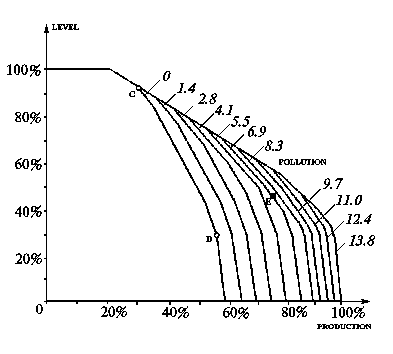
The maximal slice corresponds to the situation where restrictions on the pollution are not imposed. This slice coincides with the slice related to the restriction that equals to the maximal non-dominated value of the pollution (not greater than 13.8). The internal slice corresponds to the minimal, i.e. zero pollution. The tradeoffs curve among the production and the level of the lake shows how the level of the lake is transformed into the production.
Let us consider the zero pollution slice. For small values of the production (less than about 20%), the maximal level of the lake is feasible. Then, with the increment of the production, the feasible level of the lake starts to decrease more and more abruptly. The maximal (for zero pollution) value of the production (a little bit less, than 60%) corresponds to the minimal level of the lake. Note that it is necessarily to exchange a substantial drop of the level (more than 20% of the range in point D) for the miserable increment of the production needed to achieve the maximal value of production.
Other tradeoff curves have the same shape. It is important that the increment of the pollution results in the movement of the non-dominated frontier to the right: the feasible production values are getting larger. In contrast, feasible values of the level of the lake do not depend on the pollution value. This is a very important knowledge about the problem which may be used during negotiations.
Let us discuss in brief possible application of this decision map on the pre-negotiation stage of negotiations among inhabitants of the city, farmers and businessmen. It is supposed that everyone can receive the decision map displayed in Figure 4, or two other decision maps related to different pairs (income-pollution or level-pollution maps).
Two different zones may be identified in the decision map given in Figure 4: the zone with low values of the agricultural production (20-40%) and the zone of high production (40-100%). In the first zone, there is no conflict between the inhabitants of the city and the businessmen. In the second zone, this conflict may be started by the farmers if they will suggest to the businessmen to share the additional opportunities resulting from the pollution growth. This means that the inhabitants of the city may be interested in establishing a political coalition with businessmen. For example, they may start negotiations with the proposal of a high level of the lake. If this coalition will be strong enough, the result of negotiation may be placed around point C. Farmers may be interested to destroy the coalition. To do it, they may promise very much to the businessmen. Note that the coalition between farmers and the inhabitants has not so much sense large values of production can't be obtained without high levels of pollution.
The information discussed above, is a result of a superficial look on the decision map given in Figure 4. Additional knowledge may be obtained via detailed exploration of the decision maps. It is possible to explore three decision maps related to the problem. After it, you can identify the most preferable feasible goal. The related strategy will be constructed just at once.
Now you are invited to START the resource.