LPDO package
— Ekaterina Shemyakova 2015/02/16 14:21
This is a package for computer algebra system MAPLE. It contains symbolic algorithms for Linear Partial Differential Operators (LPDOs) and for linear Partial Differential Equations (PDEs) with parametric coefficients. We consider arbitrary LPDOs in arbitrary many independent variables and of arbitrary orders and allow coefficients to be symbolic. Numerous tools are available with the focus on the Darboux, generalized Darboux and related invariant algorithms.
Installation
To use the package, download lpdo_.txt and type
read "/home/username/path_to_file/lpdo_.txt";
(for Linux) and
read `\\path_to_file\\lpdo_.txt`;
(for Windows) at the top of your Maple sheet.
Highlights of the Package
Laplace_solver(n,E,u)
Solves E by Laplace method (not to be confused with Laplace integral method) if this is possible to do so by less or equal to n iterations. Works significantly better than existing in MAPLE PDEtools[Laplace], which fails in many examples.
- n is the number of iterations.
- E is an LPDO, that is a Linear Partial Differential Operator in the form

or a PDE, a Partial Differential Equation in the form
 .
.
Here a,b,c may depend on the independent variables. One can use any names for independent variables. When work with LPDOs, specify them using LPDO__set_vars at the top of the worksheet. For example,
LPDO__set_vars([s,t]):
would declare two independent variables s and t.
- u is optional, the dependent function.
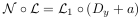
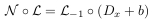
ginv(L) and ginv(L,M)
Procedure ginv(L) returns a set of generating differential invariants for L with respect to the gauge transformations
 .
.
The same procedure but with two arguments, ginv(L,M) returns a set of generating joint differential invariants for L and M with respect to the gauge transformations. Works for the following operators and pairs of operators:
 and M arbitrary LPDO.
- L is a third order LPDO given in its normalized form, i.e. for L in one of those forms.


- with principal symbol
Basic Manipulations with LPDOs
Package can work with LPDOs of arbitrary orders and depended on arbitrary many independent variables. The independent variables are to be declared at the start of each worksheet using function
LPDO__set_vars(vars):
where vars is a list of independent variables. For example,
LPDO__set_vars([x,y,z,t]):
sets 4 independent variables x,y,z,t.
Declaration
LPDO__warnings:=true:
means that using some of the function available in the package, you may get some additional information (e.g. solutions of which PDEs must belong to the field). By default
LPDO__warnings:=false:
LPDOs
 where J is a multi-index,
 , and
, and
 are kept as a one dimensional array of its coefficients.
Declaration of an LPDO and changing its coefficients.
- LPDO__create() returns an LPDO that multiplies by zero, an LPDO of order zero.
- LPDO__set_value(L::array,f,J::list) sets coefficient
 of LPDO L equaled to f.
 - LPDO__create0(a00) returns an LPDO of multiplication by a00, an LPDO of order zero.
- LPDO__create1(a10,a01,a00) returns an LPDO
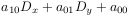 .
.
- LPDO__create2(a20,a11,a02,a10,a01,a00) returns an LPDO
 .
.
- Create_LPDO_from_coeff(a::list) returns LPDO with the coefficients from list a, in which they are
ordered lexicographically. E.g.
- Create_LPDO_from_coeff([a00,a10,a01,a20,a11,a02]) returns
- LPDO__add_value(L::array,f,J::list) adds f to the coefficient with multi-index J.
Simplification of the coefficients
- LPDO__degree(L::array) returns the order of LPDO L.
- LPDO__simplify(L::array) applies simplify to all the coefficients of LPDO L.
- LPDO__expand(L::array) applies expand to all the coefficients of LPDO L.
- LPDO__factor(L::array) applies factor to all the coefficients of LPDO L.
Algebraic operations
- LPDO__add(L1::array,L2::array) returns the sum of L1 and L2.
- LPDO__inc(L1::array,L2::array) adds L1 and L2, and save the result as L1.
- LPDO__minus(L1::array,L2::array) returns the difference of L1 and L2.
- LPDO__mult(L1::array,L2::array) returns the composition of L1 and L2
- LPDO__mult1(f,L::array) multiplies L by function f on the left.
Others
- LPDO__print(L::array) is the “pretty print”.
- LPDO__conj(L::array,g) returns the result of the gauge transformation
- LPDO__apply(L::array, f) applies L to function f.
- LPDO__value(L::array,J::list) returns the coefficient with index J, that is at D_J in L.
- LPDO__transpose(L::array) returns the formal adjoint of L.
Laplace transformations
Theory
All differential invariants of operators
with respect to the gauge transformations
can be expressed in terms of so-called Laplace invariants

If h is not zero then define a +1 Laplace transformation by equality
If k is not zero then define a -1 Laplace transformation by equality
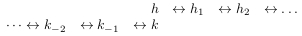
Thus until h or k are not zero, we have chain

There are some formulas relating those invariants, which implies that each new iteration of a Laplace
transformation brings us only one new invariant (only h or k is new). So, basically, we have the following chain of invariants:
The algorithm works as follows:
- computes chain of the invariants of length n into both directions
- if we meet zero on the way, then the corresponding transformed LPDO is factorizable. So we find its kernel and compute the kernel of the initial LPDO using known formulas.
Implemented procedures
- Laplace_solver(n,E,u) has been described here.
- LPDO__Lapl_trans(i,L) returns L_i, where i=1 or i=-1. LPDO L must be of the form
or
- LPDO__Lapl_chain(n,L) returns the chain of Laplace invariants and their generalizations. The chain is output in the form
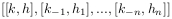
Here n is the number of iterations of Laplace transformations.
Factorization
The property of the existence of a factorization of an LPDO is invariant with respect to gauge transformations. Thus, differential invariants can be very useful for search of a factorization of an LPDO. For each type of factorization (e.g. for LPDOs with symbol (pX+qY)XY there are 12 different types of factorizations) return the conditions for the existence of a factorization for an LPDO are implemented for all bivariate LPDOs of third order in terms of generating invariants of this LPDO. More specialized notions as obstacles to factorizations are implemented too.
Darboux transformations
Classical Laplace transformations (do not confuse with Laplace transform involving integrals) are implemented. Namely, the funcitons return the resulting operators, as well as the chain of invariants for Laplace LPDOs in classical for Darboux form, that is with symbol XY, as well as for Laplace LPDOs in the form more familiar for Physicists, that is with symbol XX+YY. Construction of a Darboux transformation of order one (two) by one (two) linearly independent solutions.
Cancellation of the mixed derivatives in M from the left and from the right, for a pair (M,L) defining a Darboux transformation. Generating sets of invariants for pairs (M,L) defining a Darboux transformation unders the gauge transforamtiosn of the pairs and under the gauged evolutions. Expressions of the later in terms of the former. Invariant description of pairs (M,L) defining any at all Darboux transformation.
Invertible Darboux transformations
2015/02/16
For the first ideas on efficient and new types of invertible Darboux transformations refer to [Programming 2015 paper, to appear (part I)] and this paper (part II).
Reading the literature on Darboux transformations, one can notice only two particular cases/types of Darboux transformation:
- Levy transformations (i.e. transformations based on Wronskian formulas)
- Laplace tranformations
We discovered that there exist other types of Darboux transformations too, and among them there are many transformations with the property of invertibility. We singled out a class of such transformations that are not only invertible, but the formulas for the inverses are particular good, which make the corresponding algorithms very efficient. We call them Darboux transformations of type I.
Darboux transformations of type I
Darboux transformations of type I are those Darboux transformations (M,N) with source L and target L1 for which it is true that L=CM+f where f is an element of the field of coefficients, and C is a linear partial differential operator.
Invertible Darboux transformations represented by transformations of the gauge invariants
Not all Darboux transformations of first order are invertible. But those that are invertible, must be of type I.
For the case of operators of order three and of two independent variables we can find a generating set of all gauge differential invariants I1,I2,I3,I4,I5 (see procedure ginv here). Then the following functions allow to compute the transformations of this invariants under Darboux transformations of type I of first orders. The output is the list of new invariants.
XXY indicates that the procedure is for the operators of the form
XYS indicates that the procedure is for the operators of the form
Dx, Dy, or Dx_Dy stand for Darboux transformations with M of the corresponding principal symbol.
- LPDO__XXY_DT_with_Dy(I1,I2,I3,I4,I5)
- LPDO__XXY_DT_with_Dx(I1,I2,I3,I4,I5,r) (case I2<>I3 only)
- LPDO__XYS_DT_with_Dx(I1,I2,I3,I4,I5)
- LPDO__XYS_DT_with_Dy(I1,I2,I3,I4,I5)
- LPDO__XYS_DT_with_Dx_Dy(I1,I2,I3,I4,I5)
Orbits of Darboux transformations of type I
Darboux transformations of type I are created to be particular efficient. Implementation of orbits for operators of arbitrary kinds is work in progress. Here we implement the analogue of Laplace invariants chain for operators of the form
In the same manner as for Laplace transformations, Darboux transformations of type I are invertible. Therefore, if one element in the orbit is solvable then all the others are solvable too. Here for brevity we say that linear partial operator is solvable meaning the corresponding equation is solvable in quadratures.
- LPDO__DT_of_type_I(C,M,f) performs a step of invertible Darboux transformation of type I. Returns list [N,L1,Minv,Ninv,A,G], where N,L1 are operators from the intertwining relation NL=L1M, and Minv,Ninv are
operators defining the intertwining relation for the inverse. That is Ninv*L1=L*Minv. Operators A,G are operators that relates M and N: MA=GN (this relation is only true for invertible Darboux transformations).
- LPDO__XYS_chain_of_first_order_invertible_DTs(chain,I1,I2,I3,I4,I5) applies Darboux transformations as indicated in argument “chain” to an operator given by its gauge invariants. Argument chain should be of the form of the list, where each element indicates Darboux transformation of certain type. Thus, e.g. [1,1,2,3] indicates the sequence: Darboux transformations with principal symbol Dx, then with Dx, then with Dy, and then with Dx+Dy. The output is a list of lists: [[invariants after first Darboux tr.],[invariants after second Darboux tr.],…]
- LPDO__XYZ_Chart(b,list_of_invs) computes (including plotting) b applications of all possible Darboux transformations of order 1 of type I to an operator given by its gauge invariants. Returns list of lists: [L1,L2,L3]. L1: if used later inside command display(L1, scaling=constrained,axes=Normal), will plot the orbit, L2: list of points (D_y up, D_x right, D_x+D_y on the diagonal), L3: list of lists of invariants (in correspondence with L2)
Maple 16 worksheet example 1 (infinite orbit)
Maple 16 worksheet example 2 (9 elements orbits, "square shape")
Maple 16 worksheet example 3 (infinite orbit in one direction, "kite shape")
Equivalence-Shift procedure
- LPDO__a_step_of_Eq_and_Shift_for_Type_I(C,M,f,S,T) performs a step of Equivalence-Shift procedure for L with symbol XXY for type I so for L=CM+f
- LPDO__a_step_of_Eq_and_Shift(L,M,N,L1,Minv,Ninv,A,G,S,T) performs a step of Equivalence-Shift procedure for L of arbitrarily form. Returns [Ln,Mn,Nn,L1n,Minvn,Ninvn,An,Gn].
- LPDO__a_step_of_Eq_and_Shift_basic(L,M,N,L1,S,T) performs a step of Equivalence-Shift procedure M -> M+S*L, N -> N+L1*S for L of arbitrarily form, does not compute the auxilary operators, just the change in L and M, L1, N. Returns [Ln,Mn,Nn,L1n]